EWI Space : Project Chipsee
Image classification is used on overhead imagery to detect specific objects such as planes, cars and buildings. Creating and training effective deep learning image classification models is dependent on the proper tuning of model hyper-parameters, along with appropriate image preprocessing and standardization.Most computer vision tools process and display images as 8-bit; however, most overhead imagery is captured as 16-bit images, allotting a larger range of storage for a wider range of lighting conditions. This disparity in storage capacity raises some interesting questions about what image preprocessing and standardization steps should be taken in order to maximize model performance on overhead imagery, including:
- What is the difference in model performance between models trained on 16-bit images and models trained on images converted to 8-bit?
- How should image pixel values be standardized?
- Should standardization be based on only a collection of local or global pixel intensities?
To explore and answer these questions, we evaluated the effect of five different image standardization methods on the training and performance of a ResNet50-based image classifier trained to detect airplanes in overhead imagery.
16-bit vs. 8-bit Imagery
Within an image, digital information is stored in pixels as intensities or tones. An 8-bit image can hold 256 different intensities within a single image channel; a standard color image has 3 channels - red, green and blue (RGB). Thus, each pixel in a standard RGB image consumes 24 bits of information. In all, RGB 8-bit images can hold up to 16.7 million different values. On the other hand, 16-bit images can hold 65,536 pixel intensities in a single channel resulting in 28 billion possible values. This is a significant difference, several orders of magnitude larger, and has implications in how this data is processed.
 |
|
| 16-bit | 8-bit |
Challenges with Satellite Imagery
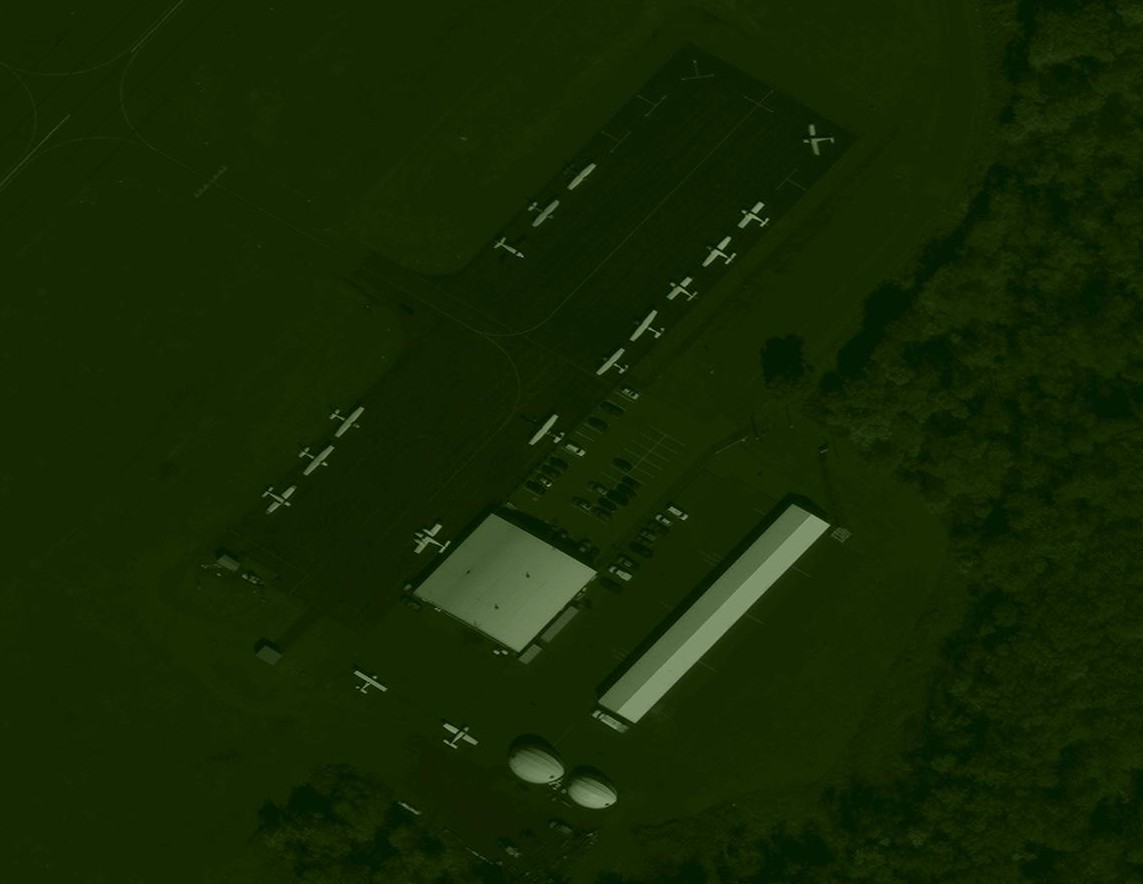
In addition to being 16-bit, satellite imagery is huge, generally on the order of tens of thousands of pixels in width and height. All images used in this blogpost are derived from the Rareplanes dataset (1) which includes panchromatic (single channel) imagery of different airports with over ten thousand labeled planes. To train an image classification model, we needed to "chip" the full images into smaller tiles that could then be converted and standardized to be fed into a model.
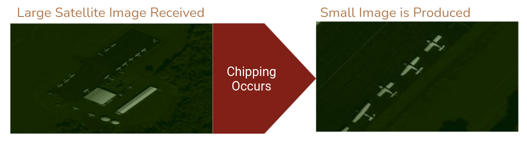 |
Image Standardization: Current Method
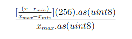
Because satellite imagery is natively 16-bit, converting those images to 8-bit may raise concerns about significant data loss. Although an entire satellite image may occupy a wide range of values across the 16-bit space, the smaller chips generated from those images likely have much less significant local variation. Thus, extracting those chips or sub-images from the satellite image may only realize a small segment of the full 16-bit range, which could then be converted into an 8-bit format without significant data loss. Currently, GA-CCRi converts 16-bit to 8-bit chips through min-max normalization where the largest pixel value in a chip is assigned to the maximum possible 8-bit value, the smallest actual pixel value is assigned to 0, and then the values are scaled between 0 and 1.
 |
This methodology extracts and standardizes only the region containing data within the 16-bit representation, and "stretches" it to use the full range of 8-bit values. This method helps to ensure that the content of the chip is visible to the human eye and generally reduces how washed out the data appears, but is it actually the optimal method for training a computer vision model to perform well on satellite imagery?
Image Standardization: Alternative Methods
We trained an airplane detector on the Rareplanes dataset (1) using five different image standardization methods: two using 16-bit imagery, and three using 16-bit converted to 8-bit imagery. The following table shows the standardized pixel range for the five different methods.
  |
  |
|
| Examples of 16-bit chips with no planes present (Cases 1/2) | Examples of 16-bit chips with planes (Cases 1/2) |
  |
  |
|
| Examples of 8-bit chip converted for Cases 3/5. | Example of 8-bit chip converted for Case 4. |
| Description | Data precision |
Standardization method |
Standardized pixel range (using example original 16-bit range of 256-10000) |
|
|---|---|---|---|---|
| Case 1 | Standardized based on the maximum 16-bit pixel intensity (65535), ignoring the actual range of pixel values in the chip. | 16-bit | 16-bit maximum | 0.0039 - 0.15258 |
| Case 2 | Standardized based on the maximum 16-bit pixel value found in the current chip. | 16-bit | Chip maximum | 0.0256 - 1.0 |
| Case 3 | Original pixel values are divided by 256 to convert to 8-bit integers, then standardized by dividing by the maximum converted pixel value. | 8-bit | Chip maximum | 0.025 - 1.0 |
| Case 4 | Original pixel values are divided by 256 to convert to 8-bit integers, then standardized based on the minimum and maximum of the converted values. | 8-bit | Image range | 0.0 - 1.0 |
| Case 5 | Original pixel values are divided by 256 to convert to 8-bit integers, then standardized by the 8-bit maximum value. | 8-bit | 8-bit maximum | 0.0039 - 0.152 |
Model Training and Evaluation
Data Generation
Using the metadata associated with each satellite image, we located the centroid of each labeled plane within each image. We then used those coordinates to create 512 x 512 chips around each plane using gdal to create our "positive" chips. "Negative" chip generation conversely used those coordinates to exclude planes entirely and only chip non-plane areas. In generating the negative chips, it is important to include as wide a variety of non-plane data as possible, to help reduce the number of false positive detections of the model. We generated one thousand 512 x 512 negative chips per positive chip.
Training
The model utilized a Resnet50 Architecture modified to accept single color imagery as input. The dataset included 187 total satellite images which were used to generate over ten thousand positive chips and one hundred and eighty thousand negative chips, all of 2562 dimensions. Each case was then trained from scratch for sixty iterations with a random split of 70% training and 30% validation for robust training. Every case has the same train and val set. Different data augmentation functions such as horizontal and vertical shifts, horizontal and vertical flips, random rotations, blurs, and crops were randomly applied throughout.
Validation
In this step we performed an initial evaluation of the model on validation data. This analysis determined the appropriate threshold a predicted probability must exceed in order to be classified as a positive. The goal was to minimize the number of false positive and false negative predictions. We used the metrics below to inform which thresholds were selected for each model.
- True Positives
- False Positives
- True Negatives
- False Negatives
- Accuracy: True Positives plus True Negatives, divided by the Total Chips
- True Positive Rate: Percent of True Positives, given a threshold.
- False Positive Rate: Percent of False Positives given a threshold. This was one of the most important metrics in determining the appropriate threshold. This often was comes at the expense of FN.
- False Negative Rate: Percent of false negative, given a threshold.
- "Augmented" False Positives: This curated metric took the the number of FPs produced from the validation set and linearly scaled that number to represent how many FPs we would expect if we were to insert a full image worth of chips into the model. Given every image is on average 65,000 x 65,000 pixels, with batch sizes of fifty or more images, there would be 85 times the size of the validation set worth of chips being processed through the model on average. Therefore, the Augmented FPs scales the number of FPs by a factor of 85.
In all five cases, the central deciding factor in threshold selection was the Augmented FP. At lower accuracy thresholds, TP rate and FN rate all do well. At thresholds close to 0, nearly all probabilities are classified as positive. Therefore the number of FN also decreases. Alternatively, FPs increase drastically by lowering the threshold. Therefore, thresholds were set at the lowest probability where the Augmented FP was below a hundred. This both satisfies a low expected FP count while optimizing accuracy, TPR and FNR. One hundred is a number that can easily be modified by a client based on individual tolerance.
Testing
- Two different testing methods were used:
- Test Method #1: Test on 512*512 chips and return one classification that details whether ANY plane exists in chip or no planes exist at all. (Does not count number of planes)
- 66 total satellite images used to generate 3798 positive chips and 61514 negative chips
- Same exact architecture used in training and validation
- Thresholds for classification determined on a case by case basis using validation set values and excel data tables
- Test Method #2: Test on full size satellite image or 15000*15000 chips of that image (whichever is smaller). Counts how many planes exist and returns visualization with plane locations highlighted.
- 66 total satellite images used to generate 180 very large chips
- CNN modified to output several probabilities based on where planes are most likely located in image
- Thresholds for classification are copied from the first testing method
- Test Method #1: Test on 512*512 chips and return one classification that details whether ANY plane exists in chip or no planes exist at all. (Does not count number of planes)
Results and visualizations:
Cases 1 and 2 show a strong statistical argument for the use of 16-bit imagery in training CNNs based on satellite imagery. Cases 1 and 2 both have the highest amount of true positives , low amounts of false negatives and a high recall score. These are important indicators for GA-CCRi which strives to detect all objects in an image. Case 2 in particular stands out as using the most optimal standardization method as it boasted a high recall score throughout testing while maintaining a low number of false positives allowing for less post-inference vetting. Please review the table below for an in-depth look at the test metrics.
| Test Method #1 | ||||||||
|---|---|---|---|---|---|---|---|---|
Case |
Threshold | TP |
FP |
TN |
FN |
Precision |
Recall |
F1- Score |
Case 1 |
0.55 | 2086 |
2 |
61512 |
1721 |
0.9990 |
0.5479 |
0.7077 |
Case 2 |
0.60 | 2115 |
3 |
61511 |
1692 |
0.9986 |
0.5556 |
0.7139 |
Case 3 |
0.65 | 2059 |
1 |
61513 |
1748 |
0.9995 |
0.5408 |
0.7019 |
Case 4 |
0.60 | 1913 |
9 |
61505 |
1894 |
0.9953 |
0.5025 |
0.6678 |
Case 5 |
0.70 | 1658 |
2 |
61512 |
2149 |
0.9988 |
0.4355 |
0.6065 |
| Test Method #2 | |||||||
|---|---|---|---|---|---|---|---|
| Case | Threshold | TP |
FP |
FN |
Precision |
Recall |
F1- Score |
| Case 1 | 0.55 | 2697 |
1635 |
8204 |
0.623 |
0.247 |
0.354 |
Case 2 |
0.60 | 2652 |
1319 |
8249 |
0.665 |
0.243 |
0.356 |
Case 3 |
0.65 | 1916 |
829 |
8985 |
0.698 |
0.176 |
0.297 |
Case 4 |
0.60 | 2023 |
1126 |
8878 |
0.642 |
0.186 |
0.288 |
Case 5 |
0.70 | 1242 |
1046 |
9659 |
0.543 |
0.114 |
0.188 |
*Bolded values indicate the best results for that metric;
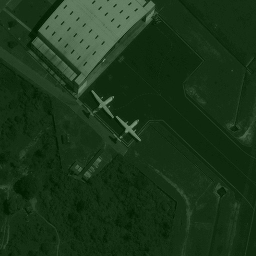
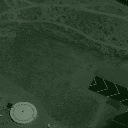
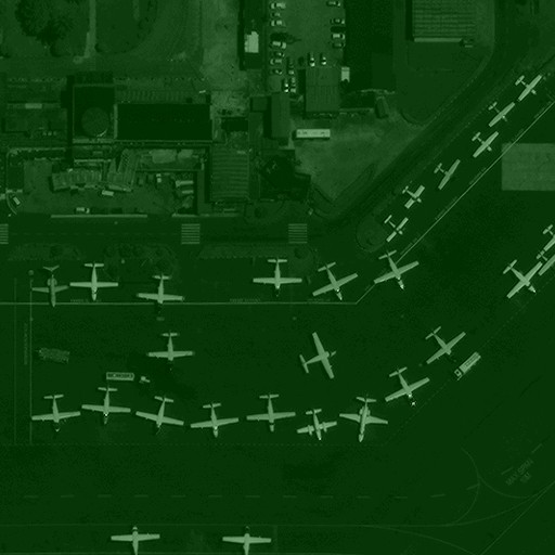
An example of output received from testing method #2 on a full size satellite image for the 5 different cases:
 |
 |
| Case 1: 0 true positives detected, 1 false positive detected. | Case 2: 8 true positives detected, 2 false positives detected. |
 |
 |
| Case 3: 2 true positives detected, 1 false positive detected. | Case 4: 5 true positives detected, 1 false positive detected. |
 |
|
| Case 5: 0 true positives detected, 1 false positive detected. |
Conclusion
Although the cost associated with using 16-bit imagery is more expensive then that of 8-bit imagery, it is clear that 16-bit imagery performs significantly better on deep learning plane detection models. Additionally, the choice of normalization and preprocessing methods employed have a significant effect on model performance. Specifically, intra-chip pixel values are potentially the best values to use during the preprocessing stage. A logical next step would be to assess whether the costs associated with these methods is worth the improvement in performance.
References
(1) Shermeyer, J., Hossler, T., Van Etten, A., Hogan, D., Lewis, R., & Kim, D. (2021). Rareplanes: Synthetic data takes flight. In Proceedings of the IEEE/CVF Winter Conference on Applications of Computer Vision (pp. 207-217).